
quantum telecommunication encryption
1 Product Overview
The near-infrared free-running single-photon detector module GW-NRFR1M is a free-running single-photon detector independently developed by our company, capable of detecting extremely weak light at the single-photon level. Its typical detection efficiency for 1550 nm single photons is 30%, with afterpulsing <7%, dark count rate <5k cps, and high-efficiency timing jitter ≤150 ps.
The GW-NRFR1M single-photon detector employs active quenching and active recovery technologies to rapidly suppress avalanche signals, reducing the module's dark counts and afterpulses. This product can be used in single-photon detection fields such as single-photon LiDAR, quantum key distribution, single-photon imaging, and fluorescence detection, featuring high speed, stability, and user-friendly interfaces. The output count pulses can provide a data source for users' subsequent optical pulse recovery and data post-processing. Additionally, the detector comes with a built-in time-to-digital converter (TDC) function, enabling real-time statistics of the input single-photon timing information and output, without requiring customers to set up an external TDC system.
1.1 Key Features
Based on InGaAs APD single-photon avalanche photodiode, the detection wavelength range is 900-1700 nm;
High Photon Detection Efficiency
Idle time is configurable
Low jitter
LVTTL Output
12V Single Power Supply
Low afterpulse probability
Free-running mode
1.2 Technical Indicators
The technical specifications of the near-infrared free-running single-photon detector module GW-NRFR1M are shown in Table 1-2.
| Serial Number | Functional Parameters | Technical Indicators | Unit |
| 1 | Number of channels | Route 1 | |
| 2 | Operating Wavelength | 900-1700 | nm |
| 3 | Operating Mode | Free Operation | |
| 4 | Cooling Time | ≤3 | min |
| 5 | Detection Efficiency | ~30% | @1550nm |
| 6 | Scheme Count | <5k | cps |
| 7 | Afterpulse Probability | <7 | % |
| 8 | Dead time | 0.2-100 | us |
| 9 | Vibration (High Efficiency) | ≤150 | ps |
| 10 | Power Supply | DC12 | V |
| 11 | Power Consumption | <20 | W |
| 12 | Control Interface | USB3.0 | |
| 13 | Optical Input Interface | FC/UPC | |
| 14 | Input and Output Interface | SMA | |
| 15 | Optical fiber core diameter | 62.5 | um |
| 16 | TDC Accuracy | 100 | ps |
| 17 | Gate Width | >100 | ns |
| 18 | Synchronous Signal Frequency | >1 | kHz |
| 19 | Operating Temperature | 0~35 | ℃ |
| 20 | Storage Temperature | -20~60 | ℃ |
| 21 | Product Dimensions | 110*100*44 | mm |
1.3 Hardware Interface
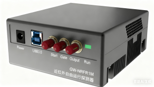
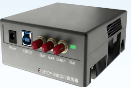
The near-infrared free-running single-photon detector module GW-NRFR1M has a total of three external interfaces, as shown in Table 1-3.
Table 1-3: GW-VIFR1M Hardware Interface
| Serial Number | Interface Name | Interface Description |
| 1 | Optic in | Fiber optic input interface, FC/PC connector; |
| 2 | Power | Module power interface, 12VDC power supply; |
| 3 | USB3.0 | Communication interface, which allows for device control, as well as TDC data export; |
| 4 | Start | The trigger input signal of the TDC is LVTTL. |
| 5 | Gate | External input signal for gate mode, LVTTL; |
| 6 | Output | Signal output interface, LVTTL. |
| 7 | Run | Work Indicator Light |
Figure 1-2: Hardware Interface Diagram (top view is the front view, bottom view is the rear view)
1.4 typical application
the field of quantum key distribution
Single-Photon LiDAR
Single-Photon LiDAR
Single-photon imaging
Photoexcitation Detection
2 Installation and Deployment
2.1 Device Power SupplyThe visible light free-running single-photon detector module GW-VIFR1M has a 12VDC power supply interface on the front panel. Connect it directly to a 12VDC power source; the interface type is a DC005-2.5mm round jack. Turning on the power supply will complete the device's power-up (please complete Section 5.4: Pre-Power-On Checks before powering on the device).
2.2 Fiber Optic Signal InputSimply connect the light source fiber output directly to the device fiber input. It should be noted that the device internally uses FC/UPC connectors, 1550nm wavelength, and 62.5µm/125µm core diameter multimode fiber, so the light source pigtail must be compatible with this. In addition, the light source wavelength needs to be between 900nm and 1700nm for the detector to respond. The light source must be attenuated to the single-photon level before being connected to the detector; otherwise, it may cause damage.
2.3 Electrical Signal OutputThe Near-Infrared Free-Running Single-Photon Detector Module GW-NRFR1M is a single-photon detector operating in free-running mode. Once the device is powered on, it generates an electrical signal output in response to optical input (under conditions with no optical input, the output electrical signal corresponds to the device's dark counts). The electrical signal output can be connected to TDC instruments, oscilloscopes, or other application devices, with the output interface being an SMA connector. Alternatively, the device can be directly connected via USB 3.0, allowing observation of photon distribution using the built-in TDC or exporting data for offline analysis.

Figure 1: Schematic diagram of electrical signal output connected to the TDC instrument
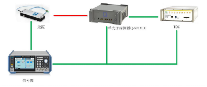
Figure 2: Schematic Diagram of Electrical Signal Output Connected to an Oscilloscope
3 Client Software
3.1 Driver Installation
(1) Power on the device and connect the computer and the device using the USB 3.0 cable;
(2) Open the computer's Device Manager, locate the device, which usually has the suffix FT601;
(3) Right-click the device, install the driver, select the driver/Win10 folder from the USB drive and install it. After a successful installation, the system will provide a prompt.
3.2 Client Software Interface
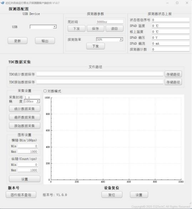
Figure 3-1: Client Software Interface
(1) Device Connection
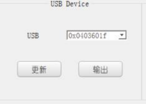
Figure 3-2: Equipment Connection Diagram
After connecting the USB, you need to click Update first. You can only click Output after the device is found. After use, you need to click Stop before unplugging the USB; otherwise, it may cause connection issues.
(2) Detector Parameters
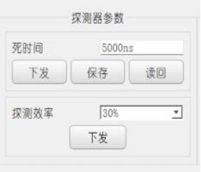
Figure 3-3: Schematic Diagram of Detector Parameters
Detector parameters are sensitive parameters, and generally only the dead time parameter is allowed to be changed;
(3) Detector Status Reporting
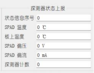
Figure 3-4: Schematic Diagram of Detector Status Reporting
Includes the parameters of the detector, mainly the board temperature, the operating temperature of the single-photon avalanche diode, bias voltage, bias current, and detector counts.
(4) TDC Data Storage
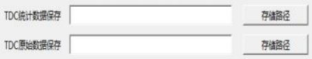
Figure 3-5: Schematic Diagram of TDC Data Storage
The data storage path of TDC can be set to a specified location.
(5) TDC Acquisition Settings
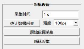
Figure 3-6: Schematic Diagram of TDC Acquisition Setup
You can choose the collection time and collection accuracy, then select whether to collect statistical distributions or raw data. You can also perform continuous collection, with the data being overlaid in the same chart.
(6) TDC Graphic Settings
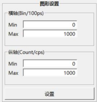
Figure 3-7: TDC Graphical Settings Diagram
The display range of the graphics can be adjusted according to actual needs, facilitating observation.
(7) TDC Data Distribution Display Region Settings
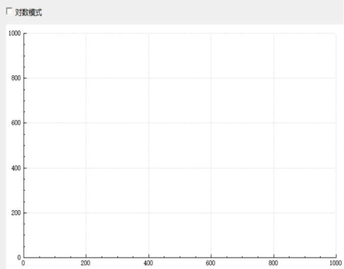
Figure 3-8: Schematic Diagram of Area Settings Displayed by TDC Data Distribution
The data distribution display area allows you to choose whether to use logarithmic mode based on actual needs.
3.3 Client Software Usage
(1) Connect the USB 3.0 cable properly and power on the device;
(2) Open the DET_Free_v1.0.7.exe software, click on Update in the USB device section, after which the USB ID number will be displayed. Click to output, and the device will be successfully connected;
(3) After selecting the storage paths for saving TDC statistical data and TDC raw data, you can start using it.
(4) After selecting the desired precision, click on data collection. The statistical data distribution will appear in the graph on the right. You can zoom in or out according to actual needs. Additionally, the collected data will be saved in the specified path.
(5) Clicking on 'Raw Data Collection' will save the original time difference data to the specified path according to the set time.
3.4 Export Data Instructions
(1) Statistical Data Collection
The GW-NRFR1M supports statistical acquisition with precision of 10 ns, 1 ns, and 100 ps. The client software collects raw data and accumulates it into a time-count distribution curve based on the configured acquisition precision, saving it in the designated folder and displaying the graph on the interface. The data stored on the PC is in .txt format. The first line of the file represents the configured acquisition precision, and from the second line onward are the accumulated counts. Each line contains two columns: the first column indicates which bin the current accumulated count belongs to, starting from 0, and the second column represents the accumulated count value within the current bin.
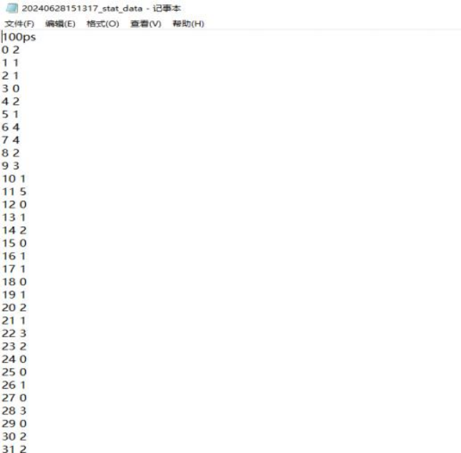
Figure 3-9: Statistical Collection Time-Count Distribution Curve Data
(2) Original Collected Data
The host computer acquires the time information of all detection events within the statistical period via USB. The statistical period can be set through the host computer. The data is saved in .txt format. The file contains two columns of data: the first column is the Start signal ID, which cycles from 0 to 65535, starting from 0 when the Start signal is received; the second column is the time difference of each detection event relative to the corresponding Start signal, measured in picoseconds (ps).
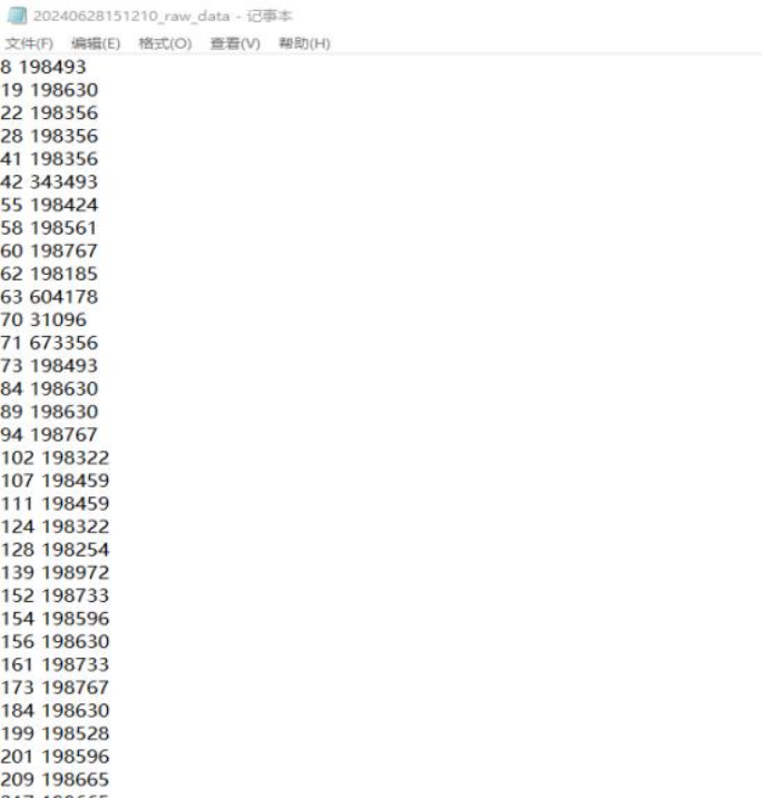
Figure 3-10: Raw Collected Data
4 Overall Dimensions
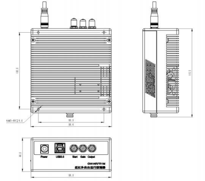
Figure 4-1: Dimensional Drawing
5 System Operation and Maintenance
5.1 Equipment Operating Environment
(1) Please operate the equipment in accordance with the installation and deployment requirements during user use to avoid damage caused by improper operation;
(2) To ensure optimal equipment performance, please use it within the specified temperature range and ensure proper ventilation for heat dissipation.
(3) Non-professionals should not disassemble the equipment.
5.2 Device Power Supply
The visible light free-running single-photon detector module GW-VIFR1M uses a 12VDC power supply. To ensure the normal operation of the device, it is recommended that the current supplied to the device be limited to 2A. To protect both the device and the safety of the operator,
It is recommended to have a reliable grounding.
(1) Power Requirements: Rated input voltage is 12V ±10%, and the input current limit is 2A;
(2) Power connection: Connect according to the requirements in Figure 3, and do not reverse the positive and negative terminals of the power supply.
5.3 Interface and Cable Connection
(1) The power supply should be connected according to the device's power wiring instructions. Note that the power supply is 12VDC, with a current limit of 2A;
(2) The output interface is an SMA interface, which detects counting pulse signals and can be connected to test equipment. The default output is LVTTL level (customizable 50-ohm output supported);
(3) The Optic in interface is a fiber optic input interface, supporting FC/UPC interface input.
5.4 Pre-Power-On Check of Equipment
(1) Place the equipment steadily and connect the wiring according to the installation and deployment requirements;
(2) The equipment is in a powered-off state during installation and deployment;
(3) The equipment cables have been connected, and the connections are correct;
(4) Pay attention to the power supply and current limitations;
(5)The peak input optical power of the detector module must not exceed 0.1mW, otherwise it may cause the probe to burn out.